
URBANITE MOBILITY DATA ANALYSIS TOOLS
Blog Urbanite -- Mobility Data Analysis.docx (sharepoint.com)
URBANITE project goal is to provide tools for the decision-making in the urban transformation field using disruptive technologies and a participatory approach. These tools should aid the process of taking decisions guiding it on data evidence. To perform these goals URBANITE offers 3 main elements:
the Social Policy Lab: to promote digital cocreation,
the Data Management Platform: related to thestorage and consumption of data,
the Decision-MakingSupportSystem: powerful processing tools to help the developing of mobility policies.
Within URBANITE the main processing tools are the simulation tools, these tools have the possibility to reproduce reality under different constraints that the ones that our cities are right now, and ever have been.These tools are very attractive because they have the power of recreating a new the MATRIX-like world where anything is possible, and any physics and traffic rule can be changed, bended or avoided. These tools allow to answer what we usually refer to the “What If Questions”.
Obviously, the mobility policy makers in our cities do not aim to change completely the way we move but they want to know what the effects of any small change are they may apply to urban mobility.To be able to simulate these small changes in the mobility policies the simulations need to feedby a lot of information related to how our cities are right now.If you do not feed real information the results of the simulation engine would differ too much being more like the mobility withinthe MATRIX.
A different set of tools with the Decision-Making Support System are tools that allow to know what the state of the city is right now, with the policies that are already implemented. These tools transform raw data in information that can be easily consumed by the policy makers. In this post, we dive into three of these tools explaining with a little bit more detail the capabilities of these elements.
Traffic Prediction Module
A citizen or public administrator could ask herself:
What is going to be the traffic like today?
Most likely the answer to this questionis:
Busy, Bad, Terrible, Dreadful, Horrendous, Awful, ...
Most people have this impression about traffic and there are a couple of reasons why so. On one side,there is a probabilistic reason: if we choose a random driver, a driver which is not a professional driver and who use her car to go to work for example,the most probable time for that person to be driving is at the time when most of the people is also driving, implying that the roads are very busy. On the other hand, there is a perception reason: if the traffic is bad, it will produce a deeper impression in our driver than otherwise. For example, if within a week the driver find herself with a traffic jam, but the rest of the days she finds free flow, is more likely that the traffic jam will be more memorable.
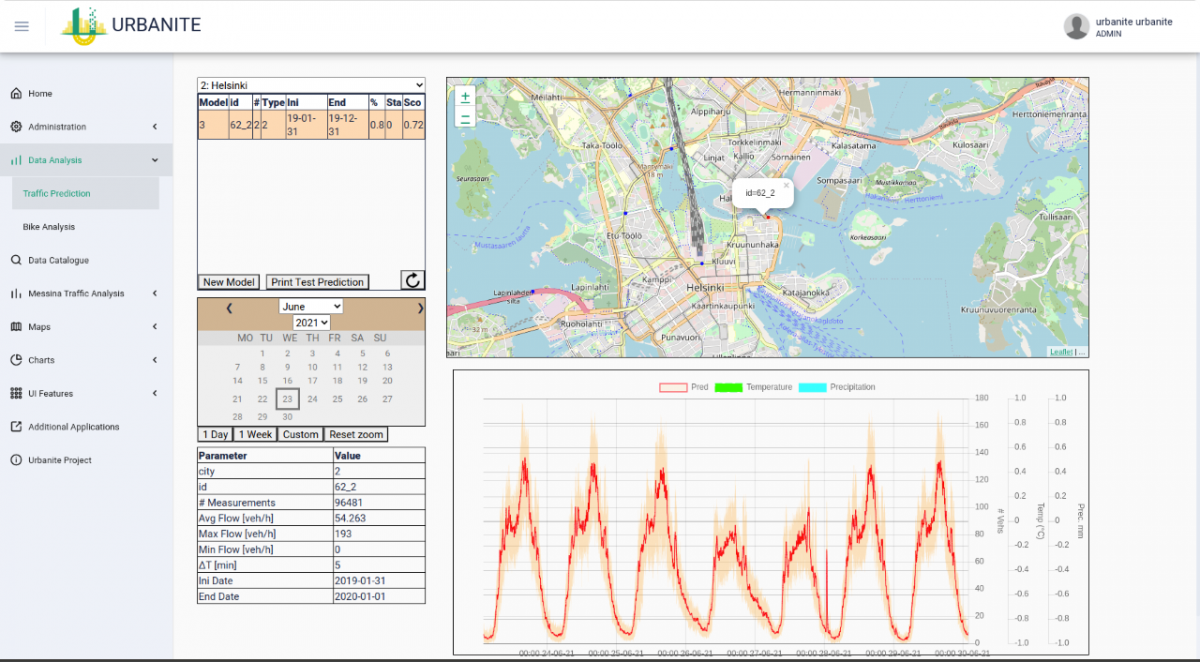
Figure 1: Detailed of the visualization for the result of the traffic flow prediction for 7 days including the confidence interval.
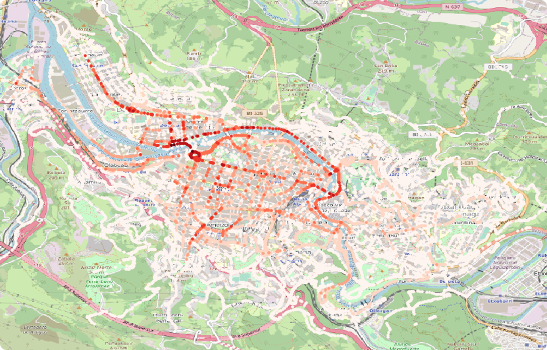
In reality, traffic flow, varies a lot according to different features, is not always as bad as the drivers perceive and if we could distribute the vehicles uniformly over the different places and times most likely the traffic would be very good. Flattening the curve of traffic flow is a chimera that cannot attained, on the contrary the traffic in our cities changes according to:
Different places within the city:there are places with way less traffic flow that other, typically these locations are points within roads with less capacity than the other because our cities have been adapted to accommodate the traffic flow in different places. The converse is also true, drivers typically, prefer high-capacity roads because they can move faster that in others.
The day of the week: Most of the locations have less traffic flow on Sundays and Saturdays than during weekdays, this is especially true for locations close to our work offices. The opposite effect can happen is locations close to leisure facilities.
The hour of the day: at night most of our roads, even the ones with higher capacity are like empty parking lot, desolate, every time I have the chance of driving by myself on a highway at night, I realise how roads are a very underutilised asset at least if you take the average over all the time.
If it is a school day, and the school buses are flooding the roads picking up our descendants in their way to learn important lessons.
If it is a bank holiday, if the main soccer team is having an exciting game, if it is rains and the roads are slippery, and many other features.
The traffic prediction tool within URBANITEallows to obtain what is the most likely traffic, for a period of time, given a set of these features.Insome sense this tool can be consider not like a predictive tool but a descriptive one.
One approach to estimate the traffic for a given set of features can be to look within the data for the last timethe set of features take the same values. Certainly,this approach has some predictive potential, but it has some drawbacks:
What if the same values of the features do not exactly fit any one within the history of the data?
What if the value of the traffic flow does not agree with other values for same features values in the historical data?
Our tool has the ability of generalize the data within the historical data to produce a viable and likely answer for the traffic. This implies the application of advanced probabilistic and other mathematical tools to the humongous amount of historic data related to traffic that is available within a given city.
OD Matrix Estimation
The OD Matrix estimation works in a similar way than the prediction module. In this case we use data from bike rental city service, specifically we consider the origins and the destinations of each one of the rentals. These are both temporally and spatially aggregated by providing the time resolution (the same way as for the traffic prediction) and by providing a set of geographic areas where to aggregate the origins and the ends of each rental.
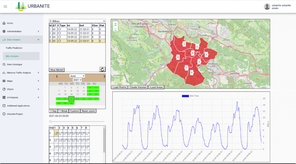
Figure 2: Integrated tool to perform OD matrix estimation for the Bilbao use case.
Trajectory Location Analysis
Finally, the last component that we explain in this communication consists in a tool able to analyze not only the origin and the destination of trajectories but also what happens in between. More specifically, and to fix ideas, we can think this tool’s goal to be obtaining the points more popular to visit in a trajectory. The processing consists in two different phases: the cleaning phase, and the aggregation phase.
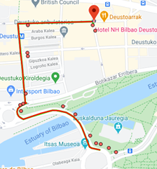
Figure 3: Result of the cleaning phase for a set of GPS points obtained from a single bike city rental in Bilbao.
The second phase, the aggregation phase, compares the points obtained in the cleaning phase for all the trajectories. Probably the simplest of these aggregations is to compute the number of times a location is visited independently of the trajectory it belongs.